AML HW3

1. 完成 value_iteration 函数, 实现值迭代算法

根据 Bellman 最优方程，我们可以得到如下的公式：

\[V^*(s) = \max_a \sum_{s'} T(s, a, s') [R(s, a, s') + \gamma V^*(s')] = \max_a Q^*(s, a) \]

可以将其写成迭代更新的方式

\[V_{k+1}(s) = \max_a \sum_{s'} T(s, a, s') [R(s, a, s') + \gamma V_k(s')] = \max_a Q_k(s, a) \]

依据如上的等式，在一次迭代的时候遍历所有的状态，找出每一个状态对应的最大估计 Q 值，然后更新 V 值，直到收敛。最终的不动点对应着最优的 V 值。

def value_iteration(env:GridWorld, gamma=0.9, theta=1e-6):"""Value iteration algorithm for solving a given environment...."""# initialize the value function and policyV = np.zeros((env.size, env.size))policy = np.zeros((env.size, env.size), dtype=int)##### Implement the value iteration algorithm hereiterations = 0while True:updated_V = V.copy()iterations += 1for now_state_x in range(env.size):for now_state_y in range(env.size):Q_values = []env.state = (now_state_x, now_state_y)for action in range(4):# get s' and rewardnext_state, reward = env.step(action=action)next_state_x, next_state_y = next_state# calc Q_valueQ_value = reward + gamma * V[next_state_x, next_state_y]Q_values.append(Q_value)# reset now_stateenv.state = (now_state_x, now_state_y)# find max Qmax_Q = max(Q_values)updated_V[now_state_x, now_state_y] = max_Qpolicy[now_state_x, now_state_y] = Q_values.index(max_Q)if np.amax(np.fabs(updated_V - V)) <= theta:print ('Value-iteration converged at iteration# %d.' %(iterations))breakelse:V = updated_V####env.reset()return policy

最终结果如下

Value-iteration converged at iteration# 154.
↓ → ↓ ↓ ↓ ↓ ↓ ↓ ↓ ↓
↓ ↓ → ↓ ↓ ↓ ↓ ↓ ↓ ↓
↓ ↓ ↓ → ↓ ↓ ↓ ↓ ↓ ↓
↓ ↓ ↓ ↓ → ↓ ↓ ↓ ↓ ↓
↓ ↓ ↓ ↓ ↓ → ↓ ↓ ↓ ↓
↓ ↓ ↓ ↓ ↓ ↓ → ↓ ↓ ↓
↓ ↓ ↓ ↓ ↓ ↓ ↓ → ↓ ↓
↓ ↓ ↓ ↓ ↓ ↓ ↓ ↓ → ↓
↓ ↓ ↓ ↓ ↓ ↓ ↓ ↓ ↓ ↓
→ → → → → → → → → ↓========== SHOW PATH ==========
(0, 0) -> (1, 0) -> (2, 0) -> (3, 0) -> (4, 0) ->
(5, 0) -> (6, 0) -> (7, 0) -> (8, 0) -> (9, 0) ->
(9, 1) -> (9, 2) -> (9, 3) -> (9, 4) -> (9, 5) ->
(9, 6) -> (9, 7) -> (9, 8) -> (9, 9)
========== END  PATH ==========

2. 完成 policy_iteration 函数, 实现策略迭代算法

从一个初始化的策略出发，先对当前的策略进行策略评估，然后改进策略，评估改进的策略，再进一步改进策略，经过不断迭代更新，直到策略收敛，这种算法被称为“策略迭代”

• Policy Evaluation

根据 Bellman 期望方程，我们可以得到如下的公式：

\[V_{k+1}(s) = \sum_{a} \pi(a|s) \sum_{s'} T(s, a, s') [R(s, a, s') + \gamma V_k(s')] \]

我们可以知道\(V^k =V^\pi\)是一个不动点

当迭代到收敛时，我们可以得到这个策略下的状态值函数

def policy_evaluation(policy:np.ndarray, env:GridWorld, gamma=0.9, theta=1e-6):"""Evaluate a policy given an environment...."""V = np.zeros((env.size, env.size))##### Implement the policy evaluation algorithm hereiterations = 0while True:iterations += 1updated_V = V.copy()for now_state_x in range(env.size):for now_state_y in range(env.size):env.state = (now_state_x, now_state_y)action = policy[now_state_x, now_state_y]next_state, reward = env.step(action=action)updated_V[now_state_x, now_state_y] = reward + gamma * V[next_state[0], next_state[1]]if np.amax(np.fabs(updated_V - V)) <= theta:V = updated_Vprint ('Policy-evaluation converged at iteration# %d.' %(iterations))breakelse:V = updated_V####return V

• Policy Improvement

假设我们在原来的状态价值函数的基础上，对于每一个状态，我们能够找到一个更优的动作\(a\), 使得\(Q^\pi (s, a) \geq V^\pi(s)\)，那么能够获得更高的回报

现在如果我们能够找到一个新的策略\(\pi'\)，使得\(V^{\pi'}(s) \geq V^\pi(s)\)，那么我们就可以得到一个更好的策略

因此我们可以贪心的选择每一个状态动作价值最大的那个动作，也就是

\[\pi'(s) = \arg \max_a Q^\pi(s, a) = \arg \max_a \sum_{s'} T(s, a, s') [R(s, a, s') + \gamma V^\pi(s')] \]

def policy_iteration(env:GridWorld, gamma=0.9, theta=1e-6):"""Perform policy iteration to find the optimal policy for a given environment...."""policy = np.zeros((env.size, env.size), dtype=int)##### Implement the policy iteration algorithm hereiterations = 0while True:iterations += 1V = policy_evaluation(policy=policy, env=env)policy_stable = Truefor now_state_x in range(env.size):for now_state_y in range(env.size):Q_values = []env.state = (now_state_x, now_state_y)for action in range(4):# get s' and rewardnext_state, reward = env.step(action=action)next_state_x, next_state_y = next_state# calc Q_valueQ_value = reward + gamma * V[next_state_x, next_state_y]Q_values.append(Q_value)# reset now_stateenv.state = (now_state_x, now_state_y)# update policymax_Q = max(Q_values)now_action = policy[now_state_x, now_state_y]new_action = Q_values.index(max_Q)if now_action != new_action:policy_stable = Falsepolicy[now_state_x, now_state_y] = Q_values.index(max_Q)if policy_stable:print ('Policy-iteration converged at iteration# %d.' %(iterations))break####env.reset()return policy

最终结果如下

Policy-evaluation converged at iteration# 133.
Policy-evaluation converged at iteration# 154.
Policy-evaluation converged at iteration# 154.
Policy-evaluation converged at iteration# 154.
Policy-evaluation converged at iteration# 154.
Policy-evaluation converged at iteration# 154.
Policy-evaluation converged at iteration# 154.
Policy-evaluation converged at iteration# 154.
Policy-evaluation converged at iteration# 154.
Policy-evaluation converged at iteration# 154.
Policy-evaluation converged at iteration# 154.
Policy-evaluation converged at iteration# 154.
Policy-evaluation converged at iteration# 154.
Policy-evaluation converged at iteration# 154.
Policy-evaluation converged at iteration# 154.
Policy-evaluation converged at iteration# 154.
Policy-evaluation converged at iteration# 154.
Policy-evaluation converged at iteration# 154.
Policy-evaluation converged at iteration# 154.
Policy-iteration converged at iteration# 19.
↓ → ↓ ↓ ↓ ↓ ↓ ↓ ↓ ↓
↓ ↓ → ↓ ↓ ↓ ↓ ↓ ↓ ↓
↓ ↓ ↓ → ↓ ↓ ↓ ↓ ↓ ↓
↓ ↓ ↓ ↓ → ↓ ↓ ↓ ↓ ↓
↓ ↓ ↓ ↓ ↓ → ↓ ↓ ↓ ↓
↓ ↓ ↓ ↓ ↓ ↓ → ↓ ↓ ↓
↓ ↓ ↓ ↓ ↓ ↓ ↓ → ↓ ↓
↓ ↓ ↓ ↓ ↓ ↓ ↓ ↓ → ↓
↓ ↓ ↓ ↓ ↓ ↓ ↓ ↓ ↓ ↓
→ → → → → → → → → ↓========== SHOW PATH ==========
(0, 0) -> (1, 0) -> (2, 0) -> (3, 0) -> (4, 0) ->
(5, 0) -> (6, 0) -> (7, 0) -> (8, 0) -> (9, 0) ->
(9, 1) -> (9, 2) -> (9, 3) -> (9, 4) -> (9, 5) ->
(9, 6) -> (9, 7) -> (9, 8) -> (9, 9)
========== END  PATH ==========

3. 完成 sarsa 和 extract_policy 函数, 实现 Sarsa 算法

一个表格由所有状态和动作组成，表格中的 Q-value 表示在某个状态下采取某个动作的价值，我们可以通过不断的更新这个表格来得到最优的策略

这个表格的值由策略决定，策略变化，表格的值也会变化

\[Q^\pi(s_t, a_t) = \mathbb{E}[R_{t} + \gamma Q^\pi(s_{t+1}, a_{t+1}) | S_t = s_t, A_t = a_t] \]

那么左右两边都是可以计算的，并且都是对 Q 值的估计，我们可以通过不断的迭代来更新这个表格

即使用观测到的\(r_t\), \(s_{t+1}\) 以及通过最优策略抽样的出的\(a_{t+1}\)，得到\(r_t + \gamma q(s_{t+1}, a_{t+1})\)

采用 TD 的思想，将\(q(s_t, a_t) = (1-\alpha) q(s_t, a_t) + \alpha r_t + \alpha\gamma q(s_{t+1}, a_{t+1})\)

SARSA 用到了五元组\((s_t, a_t, r_t, s_{t+1}, a_{t+1})\)，因此我们可以通过不断的迭代来更新这个表格

在采样最佳策略的时候，使用\(\epsilon\)-greedy 策略，即以\(\epsilon\)的概率随机选择动作，以\(1-\epsilon\)的概率选择最优动作

\[a = \begin{cases} \text{random action} & \text{with probability } \epsilon \\ \arg \max_a Q(s, a) & \text{with probability } 1-\epsilon \end{cases} \]

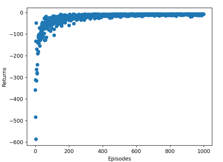
def extract_policy(q_table):"""Extract the optimal policy from the Q-value table...."""##### Implement the function to extract the optimal policy from the Q-value tablepolicy = np.argmax(q_table, axis=2)####return policydef sarsa(env:GridWorld, episodes=1000, alpha=0.1, gamma=0.9, epsilon=0.1):"""SARSA algorithm for training an agent in a given environment...."""q_table = np.zeros((env.size, env.size, 4))##### Implement the SARSA algorithm hereimport randomreturn_list = []for _ in range(episodes):x, y = env.startpolicy = extract_policy(q_table=q_table)action = policy[x, y]# 抽样if random.uniform(0, 1) <= epsilon:action = random.randint(0, 3)episode_return = 0while True:policy = extract_policy(q_table=q_table)env.state = (x, y)new_state, reward = env.step(action=action)episode_return += rewardnew_action = policy[new_state[0], new_state[1]]if random.uniform(0, 1) <= epsilon:new_action = random.randint(0, 3)q_table[x, y, action] += alpha * (reward + gamma * q_table[new_state[0], new_state[1], new_action] - q_table[x, y, action])x, y = new_stateaction = new_actionif new_state == (9, 9):breakreturn_list.append(episode_return)##### plot the returnimport matplotlib.pyplot as pltplt.scatter(range(episodes), return_list)plt.xlabel('Episodes')plt.ylabel('Returns')plt.show()env.reset()return q_table

最终实验结果如下

↓ → ↓ ↓ → → → ↓ ↓ ←
↓ ↑ → → ↓ ↓ → ↓ ↓ ↓
→ ↓ ↑ → → → ↓ → ↓ ↓
↓ ↓ ↓ ↑ → → ↓ → ↓ ↓
↓ ↓ ↓ ↓ ↑ → → → → ↓
→ ↓ ↓ ↓ ↓ ↑ → → → ↓
→ → → ↓ ↓ ↓ ↑ → → ↓
→ → → → ↓ ↓ ↓ ↑ → ↓
→ → → → ↓ → ↓ ↓ ↑ ↓
→ → → → → → → → → ↑========== SHOW PATH ==========
(0, 0) -> (1, 0) -> (2, 0) -> (2, 1) -> (3, 1) ->
(4, 1) -> (5, 1) -> (6, 1) -> (6, 2) -> (6, 3) ->
(7, 3) -> (7, 4) -> (8, 4) -> (9, 4) -> (9, 5) ->
(9, 6) -> (9, 7) -> (9, 8) -> (9, 9)
========== END  PATH ==========

4. 完成 q_learning 函数, 实现 Q-learning 算法

Q-Learning 是一种无模型的学习方法，它不需要环境的转移概率，只需要环境的奖励即可

基于 TD 的思想，我们可以通过不断的迭代来更新 Q 值

\[Q^*(s_t, a_t) = \mathbb{E}[r_t + \gamma \max_{a'} Q^*(s_{t+1}, a') | S_t = s_t, A_t = a_t] \]

\[Q(s_t, a_t) = (1-\alpha) Q(s_t, a_t) + \alpha [r_t + \gamma \max_{a'} Q(s_{t+1}, a')] \]

与 SARSA 类似，我们先通过\(\epsilon\)-greedy 策略抽样，然后更新 Q 值

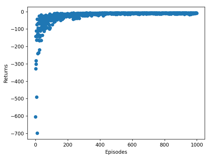
def q_learning(env:GridWorld, episodes=1000, alpha=0.1, gamma=0.9, epsilon=0.1):"""Q-learning algorithm for training an agent in a given environment...."""q_table = np.zeros((env.size, env.size, 4))##### Implement the Q-learning algorithm herereturn_list = []for _ in range(episodes):x, y = env.startepisode_return = 0while True:policy = extract_policy(q_table=q_table)action = policy[x, y]if random.uniform(0,1) <= epsilon:action = random.randint(0,3)env.state = (x, y)new_state, reward = env.step(action=action)episode_return += rewardq_table[x, y, action] += alpha * (reward + gamma *np.amax(q_table[new_state[0], new_state[1]]) - q_table[x, y, action])x, y = new_stateif new_state == env.goal:breakreturn_list.append(episode_return)####import matplotlib.pyplot as pltplt.scatter(range(episodes), return_list)plt.xlabel('Episodes')plt.ylabel('Returns')plt.show()env.reset()return q_table

最终实验结果如下：

→ → → → → ↓ ↓ → ↓ ↑
↓ ↑ → → → ↓ ↓ ↓ ↓ ↓
↓ ↓ ↑ → → → ↓ ↓ ↓ ↓
↓ ↓ ↓ ↑ → → ↓ ↓ ↓ ↓
↓ ↓ ↓ ↓ ↑ → → → ↓ ↓
→ → → ↓ ↓ ↑ → → → ↓
→ → → → ↓ ↓ ↑ → → ↓
→ → → → ↓ ↓ ↓ ↑ → ↓
↑ → → → ↓ ↓ ↓ ↓ ↑ ↓
→ → → → → → → → → ↑========== SHOW PATH ==========
(0, 0) -> (0, 1) -> (0, 2) -> (0, 3) -> (0, 4) ->
(0, 5) -> (1, 5) -> (2, 5) -> (2, 6) -> (3, 6) ->
(4, 6) -> (4, 7) -> (4, 8) -> (5, 8) -> (5, 9) ->
(6, 9) -> (7, 9) -> (8, 9) -> (9, 9)
========== END  PATH ==========

5. 结合上课所学的内容、代码实现和实验结果，分析上述四种方法的异同和优劣

相同

从模型角度（是否提供转移概率），可以从迭代公式中看出

• 有模型算法：值迭代和策略迭代
• 无模型算法：sarsa 和 q learning 算法

有模型算法能够从期望的角度计算值函数，均属于动态规划算法

于是无模型算法实际不能从期望角度来计算值函数，只能从采样的算法，而 sarsa 和 q learning 都是基于时序差分的算法来迭代

不同

对于有模型算法

• 值迭代：他是对应于每一次在当前步对最优价值函数进行估计
• 策略迭代：他对应于每一次在当前步对给定策略的价值函数进行估计，并通过贪心寻找每一个状态的最优策略

对于无模型算法

• sarsa：对当前策略的动作-状态价值函数进行估计，通过 TD 方法
• q learning：对最优的动作-状态价值函数进行估计，通过 TD 方法

优劣

• 策略迭代
  优势： 能够收敛至全局最优解，收敛速度快
  劣势： 每一次迭代都需要对所有的状态进行评估，且策略改变的时候，需要重新评估，计算量较大，从实验结果中可以看出

Policy-evaluation converged at iteration# 133.
Policy-evaluation converged at iteration# 154.
Policy-evaluation converged at iteration# 154.
Policy-evaluation converged at iteration# 154.
Policy-evaluation converged at iteration# 154.
Policy-evaluation converged at iteration# 154.
Policy-evaluation converged at iteration# 154.
Policy-evaluation converged at iteration# 154.
Policy-evaluation converged at iteration# 154.
Policy-evaluation converged at iteration# 154.
Policy-evaluation converged at iteration# 154.
Policy-evaluation converged at iteration# 154.
Policy-evaluation converged at iteration# 154.
Policy-evaluation converged at iteration# 154.
Policy-evaluation converged at iteration# 154.
Policy-evaluation converged at iteration# 154.
Policy-evaluation converged at iteration# 154.
Policy-evaluation converged at iteration# 154.
Policy-evaluation converged at iteration# 154.
Policy-iteration converged at iteration# 19.

• 值迭代

  优势： 每一次迭代只需要对所有的状态进行评估，不需要对策略进行评估，计算量较小，能收敛至全局最优解
  劣势： 对于迭代收敛速度而言，可能会比策略迭代慢一些

Value-iteration converged at iteration# 154.

• sarsa
  优势：在线学习算法，能处理环境动态变化，通过实际交互数据更新策略，收敛稳定
  劣势：收敛速度较慢，需要大量的采样，同时可能收敛至局部最优解

  

• q learning

  优势：适用于复杂环境，能处理大量状态和动作组合，更新过程简单
  劣势：需要大量的探索才能收敛，对参数选择敏感，初期表现不佳，对噪声和不稳定环境敏感，可能导致收敛问题

  

小结

值迭代和策略迭代得到的路径较一致，说明它们都能找到全局最优解。
SARSA 和 Q-learning 的路径相似，但因其在线学习特性，路径可能有波动。
SARSA 和 Q-learning 在初期表现不佳，但随着迭代次数增加，最终也能接近最优策略。

参考

动手学强化学习
深度强化学习 王树森